RELATION BETWEEN PARAMETERS AND ROOTS POSITION

(QUADRATIC)

By Dario Gonzalez Martinez

For this section, we will consider again the quadratic function

However, this time we will analyze the effects of parameters a, b and c on the roots’ position (and existence) of f(x).

The analysis that I would like to offer here is related to the approach utilized in Assignment 2 “Parabola’s Parameters Effects.” In other words, I shall utilize the relation between f(x) and the linear function:

To explain how parameters a, b and c affect the roots’ position and existence of the quadratic function f(x). Hence, it becomes appropriate to recall the Statement 1 written in Assignment 2 “Parabola’s Parameters Effects”:

Statement 1: Given a parabola and a linear function , the graph of the function h(x) = f(x) + g(x) is a parabola like , but its graph will be tangentially positioned on the linear function at x = 0. In other words, is a parabola tangent to at x = 0.

Given that Statement 1 is always true, we just need to imagine what would happen with the parabola when the line (linear function) changes its y-intercept (parameter c) and its slope (parameter b). These effects are shown below in animations 1(a) and 1(b) (see analysis in Assignment 2 for more details):

Animation 1(a) (changing parameter c)

Animation 1(b) (changing parameter b)

In order to simplify our analysis, we will consider the effects of parameter a separate from the effects of b and c. Before the effects of parameter a are being analyzed, we will consider a > 0 unless we say something different.

RELATION BETWEEN THE PARABOLA’S ROOTS AND PARAMETER c

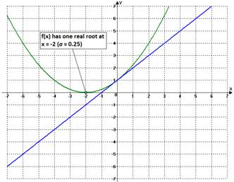
We begin with an example. Consider the function

We already know that f(x) is tangent with at x = 0. So, by reconsidering the animation 1(a), we can easily intuit that the parabola will have, at least, one real root when for some .

Figure 1

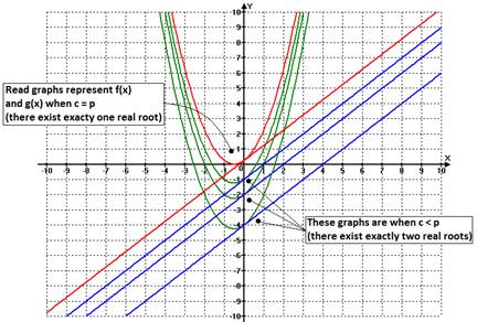
We can find p for our example by applying the discriminant “rule.” We know that a quadratic function will have one real root (double root) if and only if (this expression is called Discriminant). In other words, we need to find p such that when c = p, a = 1 and b = 1, then D = 0.

Thus, the quadratic function will have real roots if and only if .

After discussing the existence of the parabola’s roots of our example, we will discuss the location of these roots according to the variation of parameter c.

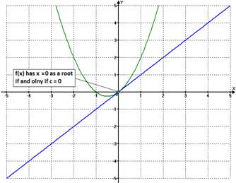
Given that the parabola is always tangent to at x = 0, the parabola will have x = 0 as a root if and only if c = 0.

Figure 2

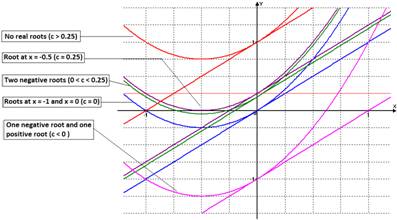
This is an important observation because we can conclude the location of the parabola’s roots by considering the values and as the “change points.” That is, by reconsider again the animation 1(a), we can easily see that if:

· f(x) has no real roots.

· f(x) has one negative root at .

· f(x) has two negative roots.

· f(x) has roots at and .

· f(x) has a negative root and a positive root.

The figure 3 below shows graphically our above summary:

Figure 3

Thus, after discussing the existence and location of our parabola’s roots, we are going to consider the graph of the expression

That is

In the XC plane drawn below:

Figure 4

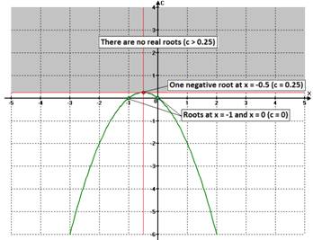
This graph gives us the relation between the location (and existence) of the roots of for different values of parameter c. We can appreciate there all what we discussed before.

RELATION BETWEEN THE PARABOLA’S ROOTS AND PARAMETER b

Now we are going to consider the following quadratic function to lead our analysis of parameter b:

We are going to remember the relation between and when b changes its value by the below animation:

Animation 2

The newly presented animation allows us to make a successful conjecture again. The existence of the parabola’s roots depend on the slope of g(x), so we can conclude that the parabola has real roots when b = r for some . Again, we can use the discriminant to find this r since we know that if a = 1, b = r and c = 1, then D = 0:

Given the seesaw effect of the linear function g(x) when its slope varies; it is reasonable having two values for b such that f(x) has one real root (double root). We can see this in figure 5 below:

Figure 5(a)	Figure 5(b)

After find the values of b that result in one real root for our parabola, we can elaborate an analysis about the existence of the roots for according to the values of b. The effect of b on the linear function is a seesaw effect; hence, the discussion of the parabola’s roots existence can be summarized as follow:

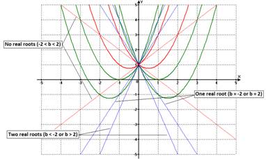
· No real roots for -2 < b < 2.

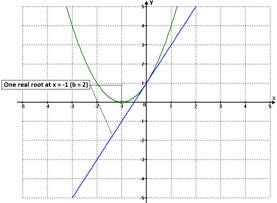
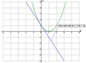
· One real root for either b = -2 (at x = 1) or b = 2 (at x =-1).

· Two real roots for either b < -2 or b > 2.

Figure 6

At the same time and given the characteristics of the parameter b effect, we can draw easily the conclusion about the location of the parabola’s roots as follow:

· Two positive roots when b < -2.

· One positive root at x = 1 when b = -2.

· One negative root at x = -1 when b = 2.

· Two negative roots when b > 2.

There is an important observation related to one of the final comments written in assignment 2, which holds:

Comment 2: The function will have a root at x = 0 if and only if c = 0.

According to the newly presented comment, we should consider the animation below:

Animation 3(a)

Animation 3(b)

We can see that as the value of b increase (more than 2), the higher negative root of the parabola is approaching to x = 0. However, x = 0 is the limit for the higher parabola’s root, so it never becomes x = 0. A similar reasoning could be drawn when the value of b decrease (less than -2) for the smaller parabola’s root. Given that c = 1 in our example, our intuition says us that having a root at x = 0 implicates that b should be infinite which does not make sense for our analysis.

Thus, after discussing the existence and location of the parabola’s roots when parameter b varies, we are going to consider the graph of the expression

That is,

In the XB plane below:

Figure 7

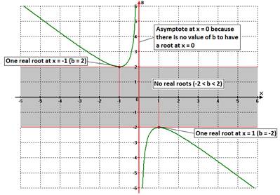
This graph gives us the relation between the location (and existence) of the roots of for different values of parameter b. Note the asymptote at x = 0, which indicates that f(x) has no root at x = 0 according to what we discussed before.

RELATION BETWEEN THE PARABOLA’S ROOTS AND PARAMETER a

Finally we are going to discuss the effect of parameter a on the parabola’s roots. In other words, we will discuss the existence and locations the parabola’s roots when parameter a varies.

Similarly to the prior analysis, we are going to start with an example. Consider the quadratic function

Once again, we need to remember the graphic effect of changing parameter a’s value and the relation with the linear function . See the animation below:

Animation 4

One more time we intuit, by observing the animation, that there is a value of parameter a which establish the “point of change” between having real roots and having no real roots for f(x).

We can check the latter intuition by considering the discriminant of f(x). Suppose that the mentioned “point of change” appears when a = s for some , then D = 0 for a = s, b = 1 and c = 1.

Therefore, when the parabola has one real root (double root) at x = -2 as it is shown in figure 8 below:

Figure 8

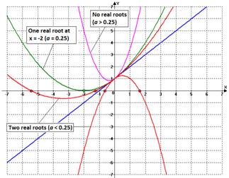
Knowing this “point of change,” we are capable to discuss the existence of the parabola’s roots related to the parameter a’s value. This analysis depends on observing what occurs to the roots in only two cases:

· When , there are no real roots.

· When , there are two distinct real roots.

Figure 9 below shows graphically our conclusion about the existence of the parabola’s roots when parameter a varies.

Figure 9

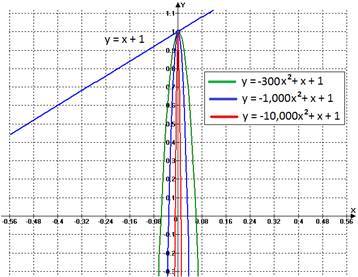
Now for the location analysis of the parabola’s roots, we should reconsider the animation 4. There we can see that the parabola’s roots are always negatives while , and if a = 0 we obtain the linear function (so, there is no parabola at all). However, the most interesting part is when a < 0. We already know, by comment 2, that the parabola cannot have a root at x = 0. Even though the parabola’s roots approximate to x = 0 (for leaf and right hand simultaneously), they are never going to be located at x = 0 because, for that to happen, our intuition tells us that a should be infinite, which does not make sense for the problem.

The figure 10 below shows what we just mentioned:

Figure 10

Therefore, in brief, we will have the following location for the parabola’s roots according to the parameter a’s value:

· One negative root if .

· Two negative roots if .

· There is no parabola if a = 0 (actually, we obtain )

· One negative root and one positive root if a < 0

Note two important observations:

Observation 1: there is no root at x = 0

Observation 2: parameter a must be nonzero real number

Thus, after discussing the existence and location of the parabola’s roots when parameter a varies, we are going to consider the graph of the expression

Or similarly,

In the XA plane below:

Figure 11

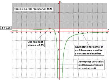
This graph gives us the relation between the location (and existence) of the roots of for different values of parameter a. Note the asymptotes at x = 0, which indicates that f(x) has no root at x = 0 according to what we discussed before, and the asymptote a = 0 because parameter a must be a nonzero real number (otherwise, there is no parabola at all).

GENERALIZATION

After our discussion about the effect of the parameters a, b and c on the parabola’s roots existence and location, we should generalize analysis for any quadratic function

Where .

We obviously know if the discriminant of the quadratic function is D < 0, there are no real roots for f(x). That is,

Generalization 1: if then has no real roots (complex roots).

Also, we already know if the discriminant of the quadratic function is D = 0, there is one real root (double root) for f(x). That is,

Generalization 2: if then has one real root.

Finally, we have the most interesting generalization when the discriminant of the quadratic function is D > 0. In other words,

Generalization 3: if then has two distinct real roots, and they are as follow in table 1:

*Remember that

and		a and b have the same sign	Two negative roots
		a and b have different signs	Two positive roots
		A positive root and a negative root
and	a and b have the same sign	A root at x = 0 and a negative root
	a and b have different signs	A root at x = 0 and a positive root
and	The roots are and
Table 1